L-17Dv3 application notes, version 1.2:

Revision notes:

Version 1.2:

Figure 3.2 changed due to slight ambiguity in caption wording.

Sections 9, 10 and 11 revised for clarity.

Version 1.1:

There are several changes to pin naming conventions in the new version of the application notes: Primarily the naming convention of the log adjusts for the linear extension pins have been changed. The L5A, L6A, L9 naming convention was historical and confusing - we have changed it so that the first (lowest power) adjust for the linear extension log adjusts is L9, followed by L10, and L11. The diagrams and tables in the application notes, as well as the new version of the test board (PC17Dv3.1) have been updated to reflect this.

The test board was updated - the preferred output DC adjust circuit is now implemented, and an error in the optional input amps feedback network was corrected. If you have purchased a PC17Dv3.0 board you may send it back to us and we will send you an updated PC17Dv3.1 board for no charge.

Additionally, Anadyne has added a discussion of dual arm units.

Table of contents:

Section 1 :  General introduction and specifications
Section 2:   Introduction to logarithmic amplifiers
Section 3:   Architecture
Section 4:   A1
Section 5:   A2 and A3
Section 6:   The logging section and tuning transfers
Section 7:   Tuning the output DC offset
Section 8:   Output amplifier
Section 9:   General guidance on pulse shapes, recovery nets
Section 10: How to remove overshoots, and improve settling time
Section 11: Recovery nets
Section 12: Temperature tuning
Section 13: Voltage regulators, bypassing
Section 14: Using the PC17Dv3.1's simple restorer
Section 15: Using the L-17D in die form, version 3 of the L2010
Section 16: Dual arm units
Section 17: Outline Dimensions, Packaging
Section 18: Sample PCB Footprint
Section 19: Final Notes

1; General Introduction and Specifications.

Anadyne Incorporated's purpose in designing the L-17D was to make a logarithmic front-end amplifier that meets or exceeds project specifications while being as easy to use as possible. In practice, this translates to low noise, low offset and drift, linear drift, low power consumption, large dynamic range, large bandwidth, and very linear log transfers for performance; and many design considerations that enable rapid and inexpensive assembly and tuning in a production environment for ease of use.

Table 1.1; Specifications:

Characteristic	Value	Notes
Package Size	Packaged: 10mm×10mm Die: 2mm×3mm
Input Rail Voltages	±5V to ±7V
Operating Temperature range	-55°C to 95°C	The L-17D is burned in under power at 150°C
Current draws at ±6V	32mA, I-, I+
Dynamic range linear input	>92dBv positive input, 80dBv negative input
Max dynamic range with tunnel diode	50dB
Max dynamic range with Schottky detector	65dB
Log linearity	Tunable to ±1/3 dB
Temperature drift	<0.5dB after adjustment
Input voltage noise	1.2nV/√Hz
Input current noise	1pA/√Hz
Risetime (10% to 90%)	8ns	With full dynamic range, faster with 2 log stages eliminated
Transit time (50% to50%)	8ns	Variation in transit time over full dynamic range can be tuned to < 2ns
Pulse to CW variation	<0.2dB	A change in pulse duration from 10 ns to 1 ms (at high duty-cycle) does not affect pulse height for DC coupled designs. For pseudo AC coupled designs 90%+ duty cycles are possible.
Fall time to 50mv output	<50ns (with recovery)
Max output voltage	VCC-2.1V
Output drive capability	80mA
Output slope	adjustable

Table 1.2; Absolute maximum ratings (NOT recommended operating conditions):

Parameter	Limits
Storage temperature	-65°C to +150°C
Operating temperature	-55°C to +125°C
Junction temperature	Up to 150°C
Rail voltages	±12V
Soldering temperature (Pinout A and B)	350°C for 60 seconds
A1 output current (pin 5)	70 mA
A1 output current (pin 34)	20 mA
A2 output current	10 mA
A3 output current	10 mA
Output driver current	80 mA, unless short circuit protection is used

Version 3 of the L-17D is currently offered in 3 packaging options: L-17D pinout A, L-17D pinout B, and the L2010 die. The pinout A and B packages are nearly identical. Pinout B has the added feature of being able to enable an output short circuit protection. Pinout A lacks this feature in order to improve its compatibility with designs using the older versions of the L17D. The die has all the functionality of pinout B and is discussed in section 15.

These application notes were prepared principally for new users of the L-17D. In general, they refer to the PC17Dv3.1 test board and the instructions for the test board are used as examples throughout these notes. With very few noted exceptions, the circuit examples in these notes and their reference designators are identical to the PC17Dv3.1 test board. The purpose of the PC board is to expedite the process of hands on familiarization with the L- 17D's performance characteristics and versatility. This experience will also facilitate the subsequent design of miniaturized PC boards using smaller components, or the design of hybrid structures for the users’ specifications.

The L-17D has features to facilitate the design of DLVA circuits using tunnel or Schottky diode microwave detectors, but it is also suitable for LADAR or any other photo-detector readout. These application notes will give many insights into tunnel and biased Schottky DLVA design, and each will be considered separately due to the different advantages and challenges each offers. Roughly, tunnel designs are usually DC coupled and have very low noise, so they benefit from a very low noise, temperature stable logarithmic amplifier. Biased Schottky detectors generate more noise and signal, so the noise contribution of the amplifier is not as significant. In addition, Schottky detectors typically have a much larger usable dynamic range and a larger useful non-square law region, so much of the extended range discussion is geared towards their use. Unfortunately, biased Schottkys have large offsets, which are temperature dependent, so they are typically used in conjunction with self-tuning baseline restorer designs. The use of zero bias Schottky detectors is not recommended because of the variation in their behavior at low power over temperature.

Anadyne Incorporated has done significant research and development into restorer design and has a variety of existing designs and custom design work for sale. These circuits allow very high duty cycles and excellent CW/signal discrimination. Please note that these restorer circuits are subject to ITAR regulations.

Figures 1.1 and 1.2 below are sample data from a simple Schottky DLVA designed to log over 50 dBm. This circuit uses a pseudo AC coupled restorer design with an Aerotech ACSP-2546PC3 detector biased with 150 µA of standing current. This data was taken with a 6 GHz input signal using a 20 MHz BW limiter on the oscilloscope. The rise and fall time of the signal was dramatically limited by the diode performance.

Figure 1.1: Sample log transfer

Figure 1.2: Sample Log Transfer errors to a well fit line with ±0.5dB boundaries

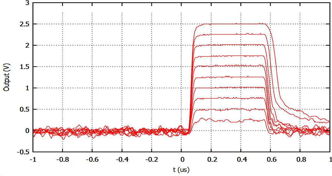
Figure 1.3: Sample Log Transfer Pulse Ladder

2; Introduction to Logarithmic Amplifiers:

For the benefit of users who are unfamiliar with log amps we have written a brief introductory section outlining the differences between log amps and the more familiar linear amplifiers.

Any front-end readout system with a large dynamic range benefits from a logarithmic compression. It displays data over a large dynamic range with equal detail. With a linear display, for example, it is impossible to see a signal that is 3 decades smaller than a second signal without changing the scale setting. Similarly, when graphing using a linear plot when data extends over several decades, any detail of the smaller valued data is unobservable.

Using a logarithmic amplifier is similar to using semi-log graph paper to enable the user to see all the data with the same accuracy. A logged signal gives all amplitudes equal weight. If measurement errors are a constant fraction of the signal, e.g.: 0.3dB, then the errors appear equal after logging.

Logarithmic compression is the most effective amplitude compression for most applications.

A few factors have to be borne in mind when using these amplifiers:

1. A log amp logs over a specified input voltage range. The lowest input voltage for which the output will be accurately related to the logarithmic output curve is called the “onset of logging input”. For inputs lower than that the output will invariably exceed that of the log of the input. Since the log(x)→ -∞ as x →0, there is a range around zero that cannot be included in the logging range. In practice for inputs between 0 and the onset of logging, the output signal is linear, starting at 0 for input 0.

2. Changing the gain of an internal amplifier before the logging section shifts the start of the logging range. This should be apparent from a fundamental property of all logarithms: Log(a*b) = Log(a) + Log(b).

3. Changing the gain of an amplifier after the logging stages changes the slope of the output. E.g., increasing the gain of the output amplifier on the L-17D by a factor of 2 will change the output slope by a factor of two from 50mV/dB to 100mV/dB.

4. The decay time of the output pulse, for pulses on the higher side of the logging range will always appear to be extremely slow. This is simply a result of the fact that you are observing the pulse settling to a part in 104, rather than a part in 100, which one can typically observe on an oscilloscope with a linear amplifier. This also means that when testing with a pulser the back edge of the pulse can look bad because pulsers do not give signals that settle cleanly and quickly to a part in 104.

5. Note that using this amplifier to take the log of a sin wave, or any function where the argument falls out of the range of logging, does not produce an output that is Vout =log(sinωt). If one did use a sin wave input, the output would be the logarithm of the input only when sinωt was positive and in the input logging range of the L-17D. When it is negative the output would be -log(|sinωt|)

See Technical Note # 1 on ANADYNE’s web site for a description of the theory of operation of the logging section.

3; Architecture:

The general internal architecture and functional pinout of the IC is presented in Fig 3.1, and the package pinout diagrams are shown in Fig 3.2. Note only one diagram is shown, but the difference between pinout A and pinout B is described in the box next to the drawing of the L-17D. The test board schematic is included throughout these app notes; a PDF of the complete schematic is provided as a separate application notes section.

L-17 Block Diagram

Figure 3.1

Fig 3.2: Pinouts for L-17Dv3

The L-17D was designed for a large variety of applications. Consequently, the ancillary circuitry for the PC17Dv3.1 test board appears complex at first sight. However, it will never be necessary to use all these components in any given application. Many, in fact, are intended to produce competing effects, such as “speedup” or “slowdown” of one or another of the amplifiers internal to the IC. Furthermore, once the optimum external circuitry for a given application and layout has been specified, almost all of the components can be preselected for subsequent units of the same type.

Typically, the L-17D is run with VCC = 6V and VEE = -6V, with a current draw of around 32 mA on each rail. However, the rails can be safely run as high as ±7V with some precautions taken in the logging section to keep the IC stable.

The IC consists of 3 cascaded linear amplifiers, A1, A2, and A3, their eight associated log stages, 3 additional linear extension log stages, and an output amplifier. The transfer curve enters the logarithmic regime when the input to the first log stage, the output of A3, reaches 20 mV. Each log stage is active for 6 dB (12dBv) for a linear input, giving an overall range of approximately 92dBv for a linear input. Both Schottky and tunnel diode detectors depart from square law behavior and roll off. Because of this, it is possible to achieve a dynamic range of 50 dBm with a single tunnel detector, and 65 dBm with a single Schottky detector, if full advantage is taken of the linear extension capability. The output amplifiers of several L-17D circuits can be summed to make extended range multi-arm units.

The start of logging depends on the gain of A1, which is programmed by an external resistor. The gains of A2 and A3 are normally ×4 and ×16 respectively, and will not need adjustment if a normal log transfer function is desired. A satisfactory transfer curve will be obtained provided that the quiescent balanced outputs of the linear amplifiers, A2 and A3, are within 3 mV of ground. Since A1's output is divided by 4 before going into a log stage, A1 could in principle be off by 10mV and the log curve would be perfectly satisfactory. However, since the amplifiers are cascaded, such a large offset of A1 is not practical.

Once you have adjusted the DC offsets of the three cascaded amplifiers you are ready to set the gain of A1 to give you the onset of logging for the input signal value you want. Simply apply the required signal level and then choose the gain of A1 so that the signal out of A3 for this input is 20 to 25 mV. The logging should not need any adjustments provided the input is linear. Finally, the log slope should be set once the output amplifier has been DC adjusted. The log slope is set by the gain of the output amplifier.

Detailed discussion of the elements of the L-17D

In this section, the general architecture of the L-17D is enumerated alongside the standard load values for the PC17Dv3.1 test board.

4; A1:

Figure 4.1: A1 and Associated Circuitry

Depending on the detector type, A1 is loaded significantly differently. Here these notes will give two separate load lists; one for tunnel diode detectors, and another for biased Schottky detectors. These are mutually exclusive and should not be confused!

Table 4.1; Tunnel input load list:

Reference Designator	Typical Value	Description
RIN-	0-15Ω	Tunnel input series resistor
RIN+	NO LOAD	Schottky input jumper
R2	NO LOAD	Used for Schottky designs
R1	300-800Ω	A1 feedback resistor, sets gain. Use a Vishay TFPT thermistor or equivalent for temperature stability of the log transfer. See section 12.
C3	2-6 pF	A1 feedback capacitor, pulse shaping, cancels input capacitance
C4	NO LOAD	Additional pulse shaping, not usually required
R7	NO LOAD	Additional pulse shaping, not usually required
R6	0Ω	Jumper to A2, some resistance is required here if using a temp comp on A2s input
R5	NO LOAD	A1 output load, not usually used
R12	50Ω	Non-inverting input DC path to ground
C10	2pF	A1 compensation
D4	NO LOAD	Diode protection; only necessary if A1 will be seeing large negative inputs.
R20	Around 7k	A1 DC adjust. See table 4.4 for values.

For Schottky operation we recommend using an input buffer amplifier. If you would like to operate a Schottky without an input amp, no amplifier should be loaded here, (U8), and 0Ω should be loaded for R27 to bypass the input amp circuitry.

We recommend a low noise, low bias current, high slew/ BW amp for the preamp (U8). Since this board has a restorer to accommodate Schottky designs, the input amplifier’s offset and drift are not relevant. The amp will not noticeably contribute to the noise seen at the output as long as it has less than input noise. The non-inverting input bias current drift of this amp should be small compared to the bias current of the Schottky detector to maintain predictable detector behavior. We have used the ADA4899 and THS4031 successfully here. The THS4031 has the advantages of slightly less quiescent current and availability in full mil temperature range packaging.

Using a Vishay TFPT linear thermistor for R1 in tunnel designs and R8 in Schottky designs almost exactly compensates for the temperature dependence of the gain in the logger, which produces the drift seen in figure 12.1. Similarly, any other PTC resistor with approximately 4000 PPM/°C temperature drift will work.

Figure 4.2: Optional Input Amplifier

Table 4.2; Schottky input load list:

Reference Designator	Typical Value	Description
RIN-	NO LOAD	Used in tunnel designs
RIN+	0Ω	Schottky input jumper
R2	50Ω	A1 feedback network
R1	200Ω	A1 feedback network
C3	2-6 pF	A1 feedback capacitor, pulse shaping, cancels input capacitance
C4	NO LOAD	Additional pulse shaping, not usually required
R7	NO LOAD	Additional pulse shaping, not usually required

Table 4.3; Schottky input amp load list

Reference Designator	Typical Value	Description
R28	50-100k	Schottky bias resistor
R30	NO LOAD	Termination resistor for pulser inputs
R27	NO LOAD	Input amp bypass
R29	50Ω	Input amp feedback
R8	330Ω (use TFPT thermistor for temperature stability)	Input amp feedback network
C11	0.1-10µF	Pseudo AC coupling capacitor. Use a low dielectric absorption
U8	ADA4899, THS4031, or equivalent	Input amplifier
C19	0.1 – 1µF	Input amp rail bypassing
C20	0.1 – 1µF	Input amp rail bypassing

This design can easily accommodate a pulser or any other 50Ω output impedance signal by loading the following: For negative incoming pulses, load A1 as if for a tunnel detector, except load 50Ω in RIN-. For positive incoming pulses, load A1 as if for a Schottky detector, except do not load the biasing resistor R28 and load a 50Ω termination resistor at R30.

As configured, this amplifier (A1) is unipolar, producing only positive outputs up to a maximum of about 3.2 Volts. It can, however, be run in either inverting or non-inverting modes. A1, and the output amplifier can be made to drive a negative voltage by adding a resistor from each of their outputs to VEE. Doing this will add to the power consumption and will be discussed shortly. A2 and A3 outputs will swing sufficiently negative without any user action.) The A1 cutoff voltage depends on the rail voltages, but it is carefully designed to be temperature independent for given VCC and VEE values. This is important for designing temperature stable recovery nets.

For tunnel diode applications, the inverting (trans-impedance) mode is far better. Tunnel diodes essentially behave as a low compliance current source and look like a 50Ω impedance for small and medium RF power inputs.

For large range tunnel circuits, it may be useful to add 10-15Ω in series with the detector because the diode's impedance drops dramatically at high RF power. This resistor effectively lowers the RF power at which A1 will limit, but otherwise this resistor is not desirable as it lowers sensitivity and increases VSWR.

Schottky diodes act as fairly high impedance voltage sources, and perform better going into the non-inverting input. Schottky designs are usually AC coupled or pseudo AC coupled because of their large input offsets and temperature drifts. Many different input topologies are possible with Schottky circuits, and a simple pseudo AC coupled circuit is included on the PC17Dv3.1 board to enable users to run Schottky detectors. Note we do not recommend the use of Zero Bias Schottky detectors

Normal A1 dominant pole compensation is 1-2 pF. Using too large a capacitor here will degrade the slew rate of the amplifier. This may be an advantage for certain setups where the variation of the transit time through the L-17D with pulse height needs to be minimized. For log amps the transit time for large pulses tends to be shorter, thus since A1 drives the higher log stages directly, it may pay to put in a larger compensation cap. So, if you want to minimize the variation in transit time, slowing the slew rats slightly can compensate for the direct path to the log section. The input capacitance, which usually gives rise to an overshoot, should be compensated by using a capacitance in parallel with the feedback resistor; its value depends on board layout, A1 gain, and detector capacitance. Typically 1-4 pF is adequate, but this value should be optimized for the particular setup. It is also possible to achieve an even flatter output by using an RC network in parallel with the feedback resistor, but this is rarely necessary. (See section 10 on pulse shaping.) However, once the designer determines the correct value for these parts, every subsequent unit will need the same value for identical performance.

A1 has a DC adjust pin and it will take about 7k to the positive rail to bring the output of A1 to ground. It is generally simpler to use the A1 DC adjust to zero A2, as zeroing A2 using A1's adjust will leave A1's output within 3mV of ground which is adequate to ensure a good log transfer. It is possible to get all of the amplifiers close enough to ground to get log linearity of <0.5dBm using just A1 DC adjust. However, it may be convenient to use the DC adjust on A3, because a very small change on the A1 adjust will dramatically change A3's output. The following table shows typical resistance values needed on the A1DC adjust pin (R20) for ±6V rails and an A1 gain of 8:

Table 4.4: A1 DC adjust reference:

A1 output offset (mV)	R20 (kΩ)
-26	8.08
-26.5	7.95
-27	7.83
-27.5	7.7
-28	7.58
-28.5	7.45
-29	7.33
-29.5	7.2
-30	7.08

A fine adjustment will probably be necessary if one nulls A3's output using the A1DC adjust.

We will discuss setting the gain on A1 in the logging section where we describe how to set up logging.

Note A1 has two outputs, pin 6 and pin 34. Pin 34 should not be loaded so that more than 20mA flow out of the pin. A1 will drive a 50Ω load, if needed, but any high current output should be taken from pin 6.

As configured, A1 will not drive a negative load. The output is an NPN emitter follower carrying about 1mA. If you require the L-17D to put out negative pulses, both A1 and the output amplifier need to have a resistor tied from their outputs to the negative rail to provide drive current. Unmodified, A1 will drive negative signals with only about 7mA, enough to drive internal loads.

A1 may require diode protection to avoid reverse biasing transistors excessively. This will happen if A1 is driven very negative and is unable to provide the current to the load so that the output limits just below zero. This can reverse bias the output transistors, causing slow degradation of transistor performance. Attaching a small signal diode to the A1 compensation pin with the anode grounded will prevent this. If the output is never driven strongly negative, this protection is unnecessary.

Do not drive A1 with pulses that exceed the input value at which A1 limits, (3.2V/Gain) by more than 3 Volts. These pulses will reverse bias the input transistors and lead to a degradation in beta. If pulses that exceed this limit may be fed into the L-17D, a clamp should be inserted before the L-17D to avoid this problem. Therefore, if you have a gain of 8 on A1, do not exceed an input voltage of 3.4V.

5; A2 and A3:

A2 and A3 have feedback networks internal to the IC and typically require minimal ancillary circuitry, signal chain jumpers, and a small amount of compensation capacitance. The additional circuitry enables a designer to slow down or speed up the amplifiers and make unusual transfer curves.

A2 has a programmable temperature stable clamp at its output. Advanced users may find programming this clamp voltage useful for temperature stable recovery nets and getting <0.4dB error log transfers.

Figure 5.1: A2

Table 5.1; A2 Load List:

Reference Designator	Typical Value	Description
C1	NO LOAD	A2 speedup
C2	NO LOAD	A2 slowdown
R4	NO LOAD	A2 gain decrease
R3	NO LOAD	A2 gain increase. Load ~2k for extremely tight log transfers.
R9	0Ω	A2 to A3 jumper
R10	NO LOAD	A2 output load
C9	1-2pF	A2 compensation
R17	NO LOAD	A2 output clamp programming resistor
R18	NO LOAD	A2 output clamp programming resistor
C5	NO LOAD	Clamp pin bypassing

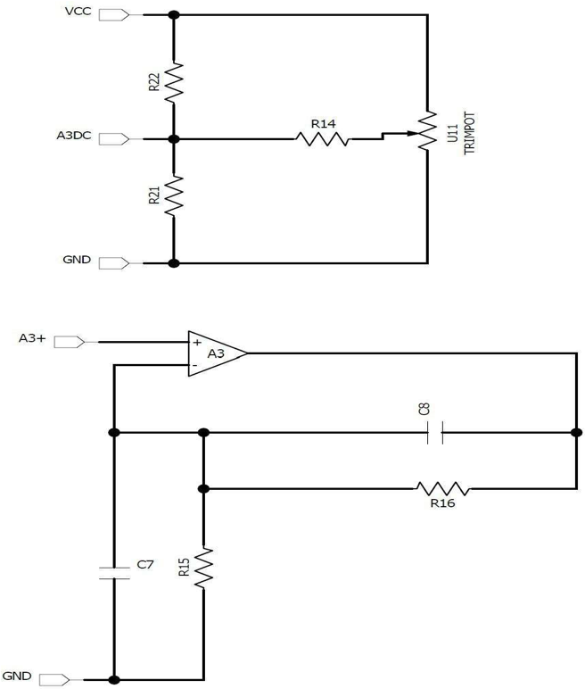
Figure 5.2: A3

Table 5.2; A3 Load list:

Reference Designator	Typical Value	Description
C7	NO LOAD	A3 speedup
C8	NO LOAD	A3 slowdown
R15	NO LOAD	A3 gain increase. (Load 2k for extremely tight log transfers.)
R16	NO LOAD	A3 gain decrease
R21	NO LOAD	A3 DC adjust
R21	NO LOAD	A3 DC adjust

The second and third amplifiers (A2 and A3) are both non-inverting, and, in general, do not need any gain adjustment. For the optimal log transfer a 2k resistor should be connected from the negative inputs of A2 and A3, pins 31 and 24 to ground. Both limit around 1.5 V. They can be slowed down by connecting capacitors from their outputs to their inverting inputs. Also, A2's compensation point is pinned out and typically needs 1-2 pF to ground to keep the amplifier from undershooting slightly. It is rarely necessary to adjust the DC of A2, since as mentioned, A2 can be zeroed using the A1 DC adjust while keeping A1's output within a couple of mv of ground which will not degrade the log linearity. A3 may need adjustment and has a DC adjustment pin. This is generally only necessary when one is trying to achieve log linearity better than ±0.5dB.

6; The Logging section and tuning transfers:

The basic principle of the logging section is described in Technical Note #1 which can be found on ANADYNE's web site. In that example, the gain is changed by a factor of 5 each time the input rises by a factor of 5. The L-17D is more accurate since the changes of gain occur every time the input increases by a factor of 4.

Figure 6.1: A simplified schematic of internal log stage circuitry

Tuning the log transfer:

It is easy to estimate the input voltage at the start of logging, as is illustrated in the following example.

If A1's gain is set to 10, the onset of logging occurs at an input voltage of Vin, which is given by:

Vin×GainA1×GainA2×GainA3=Vout

With values from previous data, this becomes:

Vin×10×4×16=20mV

Therefore, Vin=31µV.

Note with a tunnel diode the first place a voltage can be measured is at the output of A1.

For an application such as a detector log video amplifier (DLVA) using a tunnel diode with K=700, this corresponds to an input power of -43.5dBm. Note that with this setting, the overall gain, (assuming an output slope of 50mV/dB), is:

10×4×16×6.5=4160

The 6.5 factor represents the gain between the input of the log stages and the overall output, for a transfer slope of 50 mV/dB. Of course, this total gain is only valid for small signals, as the gain decreases linearly as the input signal increases in order to achieve a logarithmic transfer.

In order to shift the onset of logging to higher input powers, the gain of A1 can be reduced. However, this amplifier is very quiet and should not be run at a gain of less than 4 if TSS, (tangential signal sensitivity), is an important concern in a tunnel detector scheme. The log transfer slope depends on the output amplifier gain only.

If the input is ideal square law, it should not be necessary to use the log adjusts at all; simply adjust the start of logging by adjusting the gain of A1. For positive inputs, the range can still be extended beyond the input, which causes A1 to limit by using linear extension as described further down in this section.

Unfortunately, input devices do not always give an ideal linear input, and the L-17D has built-in adjustment pins to correct for these effects. The most common use for the log adjusts is to correct for the roll off in the response of detector diodes at high powers. The adjustment pins can also be used to generate curves that depart from a logarithmic response. A simplified schematic of a log stage is shown in figure 6.1.

If you observe that the log curve is too low above a certain input voltage, you would want to add to the output above this input. This can be done by increasing the contribution of one or more log stages to the output using the log adjusts as described below. Similarly, if a portion of the curve is too high then the appropriate log stages can be adjusted to give less of a contribution.

In order to make these corrections, it is necessary to know which log stages are operative for a given input voltage and how changing the adjusts affects the output. For a given stage, the amount of current, I, that has been delivered to the load can be determined from the following equation;

where I_max is the maximum current that a stage can deliver, and V is the voltage present at the input of the log stage.

It is basically linear up to about 20mV, and then starts to roll off. When V=50mV, I =0.76Imax, and when V =100mV, I=0.96Imax.

In general, more than one log stage is operative, since if V is going into stage n, V/4 is present at the input of stage n+1. Note that when the maximum current is being delivered for a given stage, the stage is contributing 6 dB, (12dBv) to the output. The input voltages to the log stages can be obtained by using table 6.1.

Table 6.1; Log stage input reference:

Log stage	Input voltage
Log1	A3(Vout)
Log2	A3(Vout)/4
Log3	A2(Vout)
Log4	A2(Vout)/4
Log5	A1(Vout)/4
Log6	A1(Vout)/16
Log7	A1(Vout)/64
Log8	A1(Vout)/256
Log9	Pin 11 (linear extension)
Log10	Pin 11 (linear extension) / 4
Log11	Pin 11 (linear extension) / 16

Note!: to calculate the linear extension input resistor value, note that pin 11 has 6.4k to ground internal on the chip.

Log adjusts:

Figure 6.2: PC17Dv3.1 Log adjust circuitry

Table 6.2; Logger load list:

Reference Designator	Typical Value	Description
C24	NO LOAD	High voltage stability capacitor
C25	NO LOAD	High voltage stability capacitor
C27	NO LOAD	High voltage stability capacitor
C28	NO LOAD	High voltage stability capacitor
C29	NO LOAD	High voltage stability capacitor
C30	NO LOAD	High voltage stability capacitor

There are six pins that enable you to adjust the current in a log stage, which effectively changes the log slope when this stage is active. The current into each log stage is set by an 8k resistor, which runs from -5V to VEE. Therefore, if you put an 8k resistor on a log adjust, with the other end connected to VEE, you will double the current in the log stage, and the maximum contribution to the output voltage will be the equivalent of 12dB instead of 6dB (See fig 6.2).

The current in the log stage is reduced if you connect the other end of the resistor to ground. However, when running with ±6V, an 80k resistor will cut the current in half, (since there is 5 times as much voltage across this resistor when connected to ground), and give the stage an effective contribution of 3dB. L1 adjust is usually used only for dual arm DLVA's although it can be used to improve the log linearity slightly at very low powers, and may be useful if the output voltage at TSS is specified. L6 and L7 are used to adjust for the roll off of detectors, or in matching the transfers from the two arms in a dual arm DLVA.

The linear extension is also used to compensate for the roll-off of detectors. If there is a positive polarity, low impedance input signal, it can drive the linear extension directly to extend the range beyond A1's output limit. The resistance to ground from the input to the linear extension is 6.4k. So the signal going into the first linear extension stage, L9, is simply:

For extremely robust temperature stability in the linear extension region, make a divider at the linear extension pin with impedance ~1k out of resistors that have identical temperature drift.

This board has 3 linear extension options. First, for tunnel detector applications, there is a direct linear extension (RLIN1) from the output of A1 to the 3 internal linear extension log stages.

Because Schottky diodes have a much larger range, they can utilize more linear extension techniques to get over 60dBm of logging range. RLIN2 will give a signal from the preamps output to the internal linear extension pin. This has the advantage that it has less gain than the output of A1 so it will limit at a higher input power. Finally, there is an inverting amplifier that sums the input directly into the output amplifier, giving a true linear extension. When the diode is fully rolled over and in a linear transfer region, this extension will give a very accurate transfer.

Figure 6.3: Linear Extension Circuitry

Table 6.3; Linear extension load list:

Reference Designator	Typical Value	Description
RLIN1	Tunnel diode linear
RLIN2	Schottky internal log stage linear extension
RLIN3	Schottky external direct sum linear extension
R32	5k	External linear extension amp DC path to ground
R33	5k	External linear extension amp feedback network
R34	1k	External linear extension amp feedback network
C16	5pF	External linear extension amp pulse shaping
U12	Low input bias current amplifier	External linear extension amp
C6	0.1-1µF	External linear extension amp bypassing
C12	0.1-1µF	External linear extension amp bypassing

7; Tuning the output DC offset:

The output of the logging section has a fairly large DC offset that needs to be corrected. If corrected in the obvious manner using strong trims on the output, or log DC adjusts, the logger and output amp will contribute about a ±1.5dB drift over the full military temperature range. For applications requiring less than 50C range in temperature a simple resistor from pin 19 to VCC may be stable enough to meet the users drift specs.

The output DC level is weakly dependent on the power rails so low drift regulators should be used. The recommended regulators in section 13 are stable enough to ensure temperature drift of < ±0.5dB over -55C to +95C.

The most accurate, flexible, and simplest DC offset adjustment is as follows: measure the output DC offset with the outputs of A1, A2, A3 each within a few mV of ground. Then load the following resistors on pin 8 (LOGDC):

Figure 7.1: Preferred Output DC Correction Circuit

Table 7.1 Typical Output DC Adjust Load Values

Reference	Typical Value	Description
R19	NO LOAD	LOGDC Pullup
R23	See Table 7.2	DC adjust resistor
R35	4.7K TFPT thermistor or equivalent +4000 ppm/C	DC adjust thermistor
R24	470Ω	DC adjust network
C35	0.1-1 µF	LOGDC (Pin 8) bypass

Table 7.2; Preferred Output DC Adjust Reference:

Output offset (mV)	R23 (kΩ)
-337	4.02
-384	3.92
-480	3.73
-534	3.64
-580	3.56
-637	3.48
-738	3.32
-808	3.23

The result is around a third of a dB drift at the output over the full military temperature range. With some tuning by the user, this drift can be reduced as much as desired. All subsequent units from the same wafer will need the same temperature compensation network, but each wafer may need a slightly different load. This tuning method can be extended to dual arm units; simply apply a similar adjustment to each L-17 chip.

For this discussion, an output feedback resistor of 4k resulting in an output of 40 mV/dB and ±6V rails are used. The output offsets in tables 7.2 and 7.3 need to be scaled if you use a different output gain or VCC/VEE voltages.

Note! In order to observe the actual offset at the output, you should not load the output with a 50Ω cable. Use a scope probe or voltmeter as the output amplifier will limit when trying to supply sufficient current to drive this load below about 100mV.

For applications that don't require more than 50°C temperature stability this is not a problem, and the offset can be corrected using the following method:

Non-temp corrected DC adjust: A 2.2kΩ, ±100Ω, resistor to VCC should be loaded on pin 16, the output DC adjust. Then, the output should be trimmed using a resistor from pin 19 to VEE, or a resistor from pin 8 to VEE (see table 7.2)

A resistor on pin 19 instead of pin 8 will result in less temperature drift. Pin 8 was previously S+, but now functions as the logger DC adjust.

For single arm units, here are two more methods for temperature correcting the DC offset at the output. They may be preferred to accommodate existing board layouts, but they are not as simple or precise as the preferred method shown above.

The following alternate temperature tuning methods are included for users who have existing boards that do not allow the recommended circuit above:

Alternate method 1: A 2.2kΩ, ±100Ω, (2700 ppm/C) PTC linear thermistor to VCC should be loaded on pin 16, the output DC adjust. The Panasonic ERA W, V, S series of temperature dependent resistors is perfect for this application. Alternatively use a 1.5kΩ resistor (4000ppm/C) in series with a 700Ω resistor for the DC adjust. In practice, this may be advantageous because the Vishay TFPT ~4000 ppm/C resistor series is rated to -55C whereas the Panasonic ERA W, V, S are only rated to -40C. Then, trim the output using a resistor from pin 19 to VEE (see table 7.1). The logger and output amps contribution to temperature drift will be less than ±0.25dB over the full military range.

Alternate method 2: A 2.2 kΩ, ±100Ω, (4000 ppm/C) PTC linear thermistor to VCC should be loaded on pin 16. The Vishay TFPT series is ideal for this application. There are also 3900 ppm/C Panasonic parts from the ERA W, V, S series that may work. Then, trim the output using a resistor from pin 8 to VEE (see table 7.1). The logger and output amps contribution to the temperature drift will be < ±0.5dB over the full temperature range.

Table 7.3: alternate DC adjust tuning reference:

Output Offset (mV)	Pin 19 to VEE (Ω)	Pin 8 to VEE (Ω)
-425	54.8k	256k
-450	52.7k	245k
-475	50.6k	234k
-500	48.5k	223k
-525	46.5k	214k
-550	44.2k	205k
-575	42.1k	196k
-600	40k	187k
-625	38k	177k

Note!: Table 7.2 values were taken with the following conditions: sample correction values for an output offset (after loading a 2.2kΩ resistor to VCC from pin 16) with a 4kΩ output feedback resistor (approximately 50mV/dB), VCC = 6V and VEE = -6V. Note that each tuning method calls for either a resistor from pin 8 or pin 19 to VEE, not both.

8; Output Amplifier:

Figure 8.1: Output Amplifier

Table 8.1; Output Load List:

Reference Designator	Typical Value	Description
RO1	4kΩ	Output feedback resistor, 4kΩ typically sets the output slope to 50mV/dB
RO2	0-10Ω	Load 10Ω for output short circuit protection with pinout B, otherwise load 0Ω.
RO3	See DC tuning	Output pullup
RO4	See DC tuning	Output pulldown
C22	0-4 pF	Output compensation
D3	NO LOAD	Protection Schottky if the design must accommodate large negative signals
R13	Output amplifier DC adjust 0603 load point. Review DC adjust
R26	Output amplifier DC adjust 0805 load point. Review DC adjust tuning methods.

The output amplifier takes a single ended inverted input from the logger at pin 19. Its output can drive a 50Ω load, and users of the pinout B package or die can load a short circuit protection resistor.

The gain of the output amplifier determines the slope of the log curve. With a 4kΩ feedback resistor it is essentially 4, a gain that will give an output slope of 40 mV/dB.

The amplifier is generally stable with no compensation. If you need a very fast rising pulse, the compensation should be kept below 3 pF or the slew rate will be lowered. For normal operation, a 4pF compensation capacitor should be used.

If the user wishes to observe negative polarity signals, the drive capability needs to be increased. Specifically, if a low impedance load is used, we suggest using a buffer amplifier following the output amplifier. In addition, a 6kΩ resistor from the L-17D output, pin 18 to VEE should be added.

Instructions for DC adjustment are provided in the previous section.

Note! If the output amplifier is being driven negative and limits, this will lead to excessive reverse biasing of the output transistors and a diode should be connected from the output compensation pin, pin 20, to ground with the anode grounded.

9; General guidance on pulse shapes, recovery nets:

The L-17D has a very high gain for small input pulses, so care is needed to avoid pickup, ground loops, and small imperfections in input pulses. It is crucial to avoid ground loops. Plug power supplies, pulsers, or RF generators and your oscilloscope into the same power strip. If there are any problems with pulse shape, particularly for small pulses, check that the grounding is adequate. Checks that can indicate grounding problems include the following: replace the input with a 50Ω resistor to ground and then touch the ground of the input cable to the ground of the input connector. If you observe any pulse, you have a ground problem. Similarly, if connecting the grounds of any of the instruments you are using together with a low inductance wire causes any change in pulse shape coming from the L-17D, there is a ground problem. A flat ribbon multi-strand cable, like a thin battery cable, or heavy solder wick works well for this test.

When using a scope probe, do not use a long ground connection or pickup may indicate oscillations that are not real. Typical Tektronix scope probe ground connectors are too long!

In a clean environment with good grounds, the L-17D is not sensitive, and although you may have to remove overshoots, oscillation should not be a problem, even when running with very small compensation capacitors.

A poor solder joint can often cause oscillation so one test that should be made if oscillations are seen is simply to flex the test board. If this causes changes in pulse shape, there is a strong possibility that there is a poor solder joint on the board.

Another test that should be done is to move your hand over the board, without touching any components with no input power applied, while watching the output on an oscilloscope. If you observe DC shifts, but see no oscillations on the oscilloscope, there is probably RF present near the L- 17D. This is too high a frequency to be seen on the scope but the L-17D front end transistors will function like a diode detector and will rectify it, which leads to a DC shift. The RF must be shielded.

10; How to Remove Overshoots and Improve Settling Time.

Starting with A1, make sure that the feedback and compensation capacitors are small enough to allow the maximum desired frequency. Care should be taken especially with large signals, as an excessively large compensation capacitor can slew limit the amp and cause poor rise times for large signals. If A1 is faster than needed by the user, it can be slowed down to reduce noise.

However, it is probably better to slow down A2 to limit the bandwidth. You can also put a small capacitor, (0.5-2pF), across A3's feedback, (C8 in figure 5.2).

If the rising edge of A1 is not smooth and fast settling, it can be fixed using feedback capacitors or RC networks in the feedback loop. Typically, simply adjusting the feedback capacitor will give a satisfactory pulse shape. If the output of A1 overshoots, increase the capacitance, and if the output levels out prematurely and then climbs slowly to its final value, the feedback capacitance should be decreased. This looks like a notch at the top of the front-end rise of the pulse.

If correcting the pulse shape with a simple feedback capacitor slows the amplifier down excessively, a feedback RC network is necessary. This network will not seriously affect the rise time. To see how this works, consider the inverting amplifier shown in Figure 10.1 below.

Figure 10.1: A1 in the non-inverting input mode

Figure 10.2: A1 in the inverting input mode

Let us assume the overshoot is 10% of the true pulse height without the RC net in the circuit. At early times (high frequencies) we need to reduce the overall gain by 10%. At these frequencies, Zc is small. Therefore, we need to choose R7 so that:

R7║R1 = 0.9R1

to reduce the gain by 10%. To choose C4, observe the time constant, τ, for the overshoot. Simply set R7 × C4 = τ, and the net will remove the overshoot. In practice, a stronger net is usually required because the signal seen on the oscilloscope readout is not full bandwidth and does not accurately represent the very high frequencies. Also, the derivation assumes a large open loop gain. This may not be the case at the frequencies in question and this will increase the strength needed.

For the non-inverting amplifier shown in Figure 10.2, the formula is a little more complex. If the gain is

and you want to reduce the gain to G(1- α), then you need to choose

and then choose C4 appropriately.

Of course, this method makes a linear correction. The more non-linear the defect in the pulse shape is, the more difficult it will be to correct; several RC's could be used to approximate non-linear defects. In practice this is not necessary, as any sensible board design and L-17D configuration we have seen is quite easy to tune.

11; Recovery Nets

Note this is typically not necessary if a restorer loop is being used. Diode detectors develop long tails when exposed to high power inputs, particularly if the high power is applied for a long time. This leads to long settling times for the DLVA.

Fortunately, there is a simple cure for this if a log amp is being used. It is somewhat tedious the first time you do it but once you have found the correct nets for your detector, you can simply use the same values for all your units.

Suppose we have a pulse similar to the one in Figure 11.1. If we were using a linear amplifier any attempt to remove the tail of this pulse by inserting a high pass filter, for example, would induce an overshoot in the front of the pulse, and a mirror image of the undershoot at the back.

However, for a logarithmic amplifier, the gain at the top of the pulse is far smaller than the gain when the output is near ground, as in the tail, so the undershoot on the top is not seen, particularly if the tail after the pulse only shows for very large pulses. The tail seen at the back of the pulse is not a simple exponential, but it can be approximated by a sum of exponential pulses, and an exponentially decaying pulse can be removed using the circuit shown in Figure 11.2. Note this is very similar to what we were doing in the pulse shaping section with the R and C in parallel with the feedback. It is actually the inverse of that process, since we want to induce an overshoot on the front end and an undershoot after the pulse as opposed to removing an overshoot at the top and undershoot after the pulse.

Figure 11.1: Pulse with Tail

Note in figure 11.1 the tail looks large because the logged output has much more gain near ground than near the top of the pulse. If one observes the output of A1, a linear amplifier, we do not see the tail. Therefore, we need only a very small change in feedback to remove the tail.

There are two problems to solve, firstly getting the right combination of exponentials to approximate the tail, and secondly choosing the right values to undershoot the pulse the correct amount for each exponential we wish to remove. The second step involves getting the correct magnitude and time constant. Getting the correct exponentials to approximate the tail is not easy and we will describe a practical approach to eliminate the tail. However, it does help to understand how one eliminates an exponential tail before attempting the general case. It will give the user an idea of what values to use for the nets to start with.

Figure 11.2: A Single Recovery Net on A1

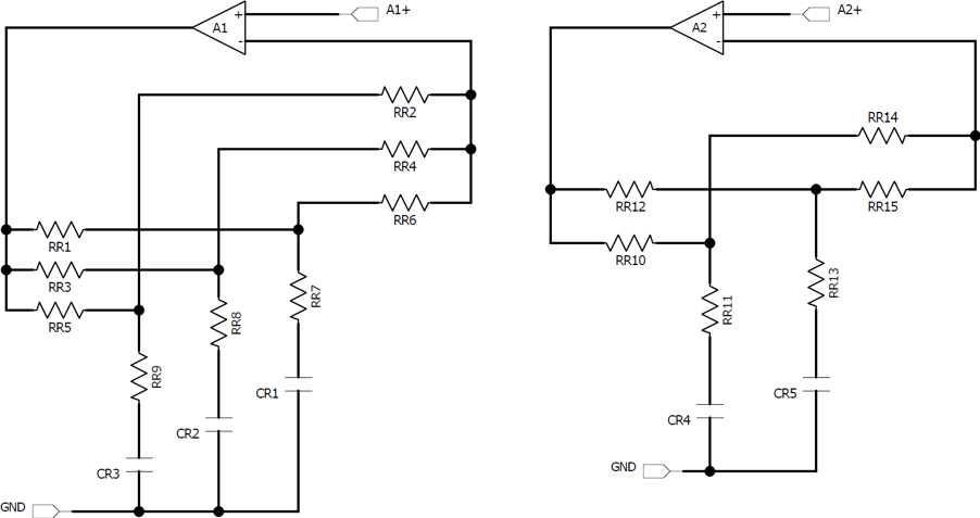
Figure 11.3: Recovery Nets on the PC17Dv3.1 Board

To find the best values for the resistors and capacitors shown in Figs 11.2 and

11.3 to cancel the overshoot due to an exponential, follow the procedure below. If we choose RR1 and RR7 to be << RR6, the time constant, τ, for the circuit is:

τ = CR1(RR1+RR7)

The magnitude of RR6 can be calculated from the relationship;

where Vo is the pulse height on the linear amplifier at t1 where the net is being applied, Vu is the desired undershoot at that amplifier output at t1, and

Note on the choice of RR7 and RR1. By making λ larger you can reduce the value of RR6. While you do want RR1 and RR7 to be much smaller than RR6, as assumed in the derivation of the formulae above, you do not want RR6 to be too big or stray capacitance will tend to shunt it out at high frequencies. Note you cannot see the tail on the linear amplifier so you do not know how big to make Vu. You can do the following to determine it. Set the RF power to that at which the pulse height at the output of the L-17 is the same as that of the exponential you are trying to cancel at the output of the L17. Measure the output of A1 at that power to get Vu. If it is too small to measure, increase the RF power by 10dB to measure the output of A1. Since the detector is still in the Square Law regime you can divide the new value of A1 by 10 to get Vu. Vo is simply the value of A1’s output at full power. When installing nets on A2 use the same procedure except look at A2’s output instead of A1’s.

To remove a real tail, proceed as described below:

Suppose your requirement is that the signal must be below 100 mV within 1 µs of the pulse ending. You measure 300 mV at a time t1 after the pulse has ended.

Choose RR7 and RR1 to make λ about 1/3. Put in CRR1 to give a time constant equal to t1. Then using the value of the tail at that time, calculate the required value for RR6 as described above for a single exponential, and put a multi-turn pot in for RR6 set to this value. Adjust the pot so it removes the end of the tail satisfactorily, checking that it does not give an undershoot at earlier times or at lower powers. If it does undershoot at lower powers, increase the value of the pot until it stops undershooting. You may have to change the capacitor when you adjust the pot. Once you have as much of the late part of the tail removed as you can with the first net, proceed to install the second net, using the same procedure to bring down the residual tail for times earlier than t1. Leave the first pot in place while adding the second and third net as it may have to be readjusted after you add the second and third nets.

After installing the second net you might have to weaken the first net slightly. Install as many nets as necessary to achieve the recovery time you need.

When installing nets on A2 look at the output of A2, just as you did with A1 to choose the A1 net values. This procedure sounds tedious, and it is until you get some experience doing it. However, customers have achieved recovery times less than 50ns with these nets.

12; Temperature tuning:

Temperature tuning is generally easy provided the drifts are linear. In the case of a log amp which works in the same manner as the L-17D there is a subtle point that needs to be addressed. The logging section uses undegenerated differential pairs (see Fig 6.1), and while we stated earlier that the current which is switched is proportional to tanh(Vin/50mV), this is only true at room temperature. More generally it is proportional to tanh(qVin/KT), where q and K are constants and T is the temperature in Kelvin. Therfore, as the temperature decreases, the current is shifted at lower input voltages, and logging starts at a lower input voltage. Essentially, the gain of the differential pairs increases as temperature decreases. Because this gain is before summation, it is equivalent to changing the gain of the A1-A3 amplifier chain. Once the input is in the logging range, the slopes are independent of temperature, as the logger is designed to keep the slope constant over temperature. There is simply a shift, as shown in figure 12.1, which assumes no temperature drift in A1, A2, or A3. The consequences of this temperature dependent gain in the logger is either; the output remains constant over temperature with no input, in which case the readings in the logging range will vary over temperature, or; if you temperature tune the unit to cancel the shift in the logging range, the output baseline will drift with no input signal.

Fig 12.1; Log Transfer Curve Shown at 3 Temperatures

Luckily a 4000 ppm/C linear PTC thermistor on A1's feedback will almost exactly cancel this change. If a linear extension signal is taken before A1, the temperature sensitive gain setting resistor should be put on the preamp in the signal chain or on that linear extension signal also. We recommend using the Vishay TPFT series resistors for this application.

Note that if you have a linear temperature change in the gain of any RF amplifiers in front of the L17, or in your detector, you can compensate for them by using an appropriate value thermistor to cure both these and the effect discussed above.

Figure 12.2: PC17Dv3.1 Temperature Tuning Provisions

If the L-17D is being used with a tunnel diode and is DC coupled, then it is necessary to trim the temperature drift in A1 so that the output of A3 remains within 3mV of ground as the temperature varies. If a baseline restorer is being used, then this is unnecessary. The procedure is simple but one detail in the procedure must be followed or it will take substantially longer than necessary to achieve satisfactory compensation.

Figure 12.2 represents what is on the test board. The diodes can be replaced by temperature dependent resistors as illustrated below in Figure 12.3. It is easier to use the temperature dependent resistors, so we show a calculation based on the use of 4000ppm/C positive temperature coefficient resistors.

Figure 12.3: Temperature Correction

Let us suppose the output of A3 is drifting by dV3/dT, and is decreasing as T increases. Also let the gain of A1 be G. We need to apply a voltage that increases with temperature to the positive input to counter this.

The magnitude needs to be V3/64G per °C to counter the observed drift. In general, there will be a 50Ω resistor to ground at the positive input to A1. Figure 12.3 shows the connections and let us assume that G=8 for simplicity. Thus, the drift referred to the input of A1 is V3/512V per °C. Assume we have a positive temperature coefficient resistor set, with a drift of 4000ppm/C, and we wish to counter this.

Suppose a 100Ω temperature dependent resistor is loaded for RT. We need to calculate the correct value of R so that the input voltage increases at the rate V3/512V.

If we connect RT and R from the positive input to A1 to VCC, and VCC=6V, then

where (RT+R) >> 50Ω

(12.1)

(12.2)

If we observe a drift at the output of A3 of say -1mv/C, then to compensate for this, we need

Substituting this for dV3/dT in equation 12.1, using equation 12.2, and setting RT=100 we get:

Solving for R, we get R = 7.75kΩ

However, installing these resistors will shift A1's DC level and we have to restore the output levels of A1, A2 and A3. Don’t try to restore the DC using the A1adjust!!! This is because the drift depends on the input offset, and adding RT and R has changed this offset. You have to restore the original offset by adding the resistor RR from the positive input of A1 to the negative rail. So carefully note the voltage at A3 before adding R and RT and then restore it by adding the appropriate value for RR. If this is done correctly, the temperature drift will go away. The appropriate resistor should be very close to RT+R, since Vin is always very small compared to VCC.

As illustrated on the test board figure, Figure 12.2, a diode can be used in place of RT, provided you know the temperature drift of the diode. Note this depends on the current density in the diode, so you should measure it with about the same current flowing through as it will carry when mounted. It is probably simpler to use the positive temperature coefficient resistors, and they can be loaded on the test board in place of the diodes if you buy them in 0603 packages.

13; Voltage regulators, bypassing:

While the L-17D amplifiers have very good power supply rejection ratio, the circuit has so much gain that it is sensitive to drifts in the power supplies.

This is especially important for DC coupled designs that do not have active restorer circuits to keep the high gain amplifier chain nulled over a large temperature range.

Figure 13.1: PC17Dv3.1 Voltage Regulator Schematic

This test board utilizes the LT1763 and LT1175 voltage regulators. These were chosen for their full military temperature range rating, miniature packaging options, and temperature stability. The datasheets for these parts recommend a very high impedance programming network (around 250k) for micropower applications; however, to maintain temperature stability, a much lower impedance network should be used (less than 6k).

We recommend using ±6V VCC/VEE voltages. The L-17D is stable up to ±7V, but the logger stabilizing capacitors in the logger section must be loaded for rail voltages over 6.2V in magnitude.

Table 13.1; Voltage regulator load list:

Reference Designator	Typical Value	Description
VR1	LT1763	SOIC package
VR2	LT1175	SOIC package
C17	0.01µF	bypassing
C14	33µF tantalum	Input power line
C13	33µF tantalum	Input power line
C18	33µF tantalum	VEE powerplane
C33	33µF tantalum	VCC powerplane
C31	0.1-1µF ceramic	High frequency power plane bypassing
C32	0.1-1µF ceramic	High frequency power plane bypassing
RV1	See voltage regulator	VCC programming
RV2	See voltage regulator	VCC programming
RV3	See voltage regulator	VEE programming
RV4	See voltage regulator	VEE programming

The L-17D has an enormous gain bandwidth product and requires robust bypassing. The rails should be bypassed with >20µF capacitors, and the L-17D power pins should have 0.1-1µF bypassing as close to the pins as possible. On the PC17Dv3.1 board, the L-17D's bypassing capacitor load points are integrated into the L-17D landing pattern and do not have their

own designators. These caps should be loaded directly onto the pins of the L-17D in a similar fashion to previous boards. Figure 13.2 shows the locations of the L-17 bypassing caps on the landing footprint. 0402 or 0603 sized 0.1 – 1.0µF caps should be loaded to ensure stable operation.

Figure 13.2: L-17D Bypass Locations

14; Using the PC17Dv3.1's simple restorer:

The PC17Dv3.1 includes a restorer design, mainly to accommodate Schottky test units. However, the restorer can also be used with tunnel input topologies.

This simple restorer design will automatically null the A1,2,3 amplifier chain, while allowing pulses under a certain width with minimal distortion, and passing upwards of a 90% duty cycle with minimal output amplitude error. To tune this circuit for a specific design takes some experience; a full discourse on restorer tuning is far beyond the scope of this document. Here

we present a standard load that passes 5µs pulses. If you would like help with restorer design contact Anadyne Incorporated. We have patent- pending restoration circuits that dramatically exceed the performance of this circuit.

The amplifiers G1 and G2 should be medium bandwidth, high slew, low offset, and low drift for optimal performance.

If a simple AC coupled Schottky detector is adequate, only the resistor R12 needs to be loaded. The input RC time constant will then be R12×C11.

Figure 14.1: PC17Dv3.1 Restorer Schematic

For a Schottky input, the pseudo AC coupling capacitor C11 acts as the high pass filter in the restorer.

Table 14.1; Schottky Restorer Load Values:

Reference Designator	Typical Value	Description
C11	3µF	Pseudo AC coupling
C15	NO LOAD	Used for tunnel detector restorer circuit
R12	NO LOAD	Used for simple AC
RG1	1k
RG3	1k
RG2	4k
RG4	50k	Determines pseudo AC couple time constant with C11
RG5	500Ω
RG6	1.5k
RG7	20k
D1	Small signal diode
R31	0-10Ω
D2	Schottky diode
G1	>20 MHz precision op
C21	0.1-1µF	G1 rail bypassing
C26	0.1-1µF	G1 rail bypassing
G2	>20 MHz precision op
C14	0.1-1µF	G2 rail bypassing
C23	0.1-1µF	G2 rail bypassing

Table 14.2; Tunnel Restorer Load Values:

Reference Designator	Typical Value	Description
C11	NO LOAD
C15	3µF	Pseudo AC coupling time
R12	NO LOAD
RG1	1k
RG3	1k
RG2	10k
RG4	500k	Pseudo AC coupling time
RG5	500Ω
RG6	1.5k
RG7	20k
D1	Small signal diode
R31	NO LOAD
D2	NO LOAD
G1	>20 MHz precision op
C21	0.1-1µF	G1 rail bypassing
C26	0.1-1µF	G1 rail bypassing
G2	>20 MHz precision op
C14	0.1-1µF	G2 rail bypassing
C23	0.1-1µF	G2 rail bypassing

The duty cycle circuit on these restorers (RG5, RG6, RG7, D1, G2) is very sensitive and may need tuning depending on how much gain A1 has, the bandwidth of G2, and how much noise is present at the input of the L-17.

15; Using the L-17D in die form, version 3 of the L2010:

Some customers prefer to use version 3 of the L-2010 die in their designs rather than the packaged L-17D part. The advice in for the packaged L17-D in this document is largely applicable using the following diagram (Fig. 15.1):

Figure 15.1: L-2010 Die Drawing

Table 15.1; Pad coordinates:

Pad coordinates:	x (µm)	y (µm)
A2comp	336	128
A1O2	496	128
A1inM	656	128
CLAdj	816	128
A1comp	976	128
A1+	1136	128
A1DC	1296	128
A1BP	1564	128
L11Adj	1724	128
Vee	1908	732
A1out1	1904	892
VCC	1904	1093
LogDC	1904	1504
L1Adj	1904	1664
L7adj	1904	1824
LIN	1904	2144
GND3	1904	2304
L6Adj	1904	2464
VEE(sub)	1904	2624
L9Adj	1664	2920
ODC	1504	2920
AuxO	1344	2920
O	1184	2920
Oprot	1024	2920
Oinm	864	2920
Ocomp	704	2920
L10Adj	544	2920
VEE2	384	2920
VCC2	128	2292
A3INM	128	2132
A3DC	128	1972
A3O	128	1812
GND2	128	1652
A3INP	128	1492
A2O	128	1332
GND1	128	1172
A2INM	128	852
A2INP	128	224

L-2010 die are not burned in under power like L-17D chips, so some offset drift settling is possible. We encourage die customers who are concerned with offset drifts, (mainly applicable in DC coupled units), to burn in their units under power before trimming for production parts.

Some of the recommended load values will be slightly different when using die to account for the missing package parasitics. For example, if the LogDC pad is not bonded out, it does not need a bypassing capacitor. Also, the output amplifiers feedback resistor often needs 1-2pF in parallel with it to give a good output pulse shape for units utilizing L2010 die bonded directly to micro PC boards or hybrid substrates. As for the packaged part designs, once the appropriate values are determined for a board layout, they will remain the same for all subsequent units.

To use the output short circuit protection circuit, use an identical resistor network as is used in the PC17Dv3.1 test board. To use the output without short circuit protection, the O (output) and OProt pads must be bonded out and shorted together.

16; Dual arm units:

Because the logger output on the L-17Dv3 is now single ended and inverted, several L17-D outputs can be summed into a single output amplifier. Pin 19 is the inverted logged output in series with 1k. For any L-17D chips whose output amplifiers are inactive, we recommend grounding pin 20 (output compensation) and short pin 17 and 18 together if using pinout B or die, to disable the unused output amplifier. Pin 19 can be summed into another L- 17D's output amplifier or another external driver if the user desires.

17; Outline Dimensions, Packaging:

Package Dimensions:

For L-17D#A and L-17D#B parts.

Figure 17.1

Typical dimensions in inches.

Part Labeling:

Figure 17.2

Notes: #A pinout shown here. This labeling convention effective November 2018.

Shipping Packaging:

Figure 17.3

Notes: L-17D parts are shipped in conductive plastic packaging with soft conductive foam padding, with up to 30 parts per box in the above arrangement unless instructions are given and agreed upon ahead of time.

Typical dimensions in inches.

18; Sample PCB Footprint:

Figure 18.1

Note: Customers will often generate a jig to bend the L-17D legs to fit the holes in their footprint. Some customers use the L-17D packaged part as a surface mount component instead of feeding the pins through holes in the board with no adverse effects in high reliability applications. Typical dimensions in inches.

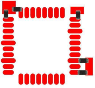
Figure 18.2

Sample Bypassing Locations.

19; Final notes:

Good luck with your projects. Anadyne Inc. is happy to answer any questions customers have and help generally with design problems. Check the Anadyne website for the latest versions of the L-17D application notes, useful technical notes and articles, test-board documentation, technical support and contact information, and available products.